Simple example of how to use NSEpy with backtrader #

This is a simple example to show how you can use P/E ratio to make investment decision. Our investment of choice is NIFTY index for simplicity (Though you cannot invest directly in the NIFTY, you can invest in any one of 11 Exchange traded funds which are based on NIFTY)

Lets get into tools and strategies now. To downloading index historical data we are going to use NSEpy. For back-testing our strategy we are using backtrader. Install dependencies - pip install nsepy backtrader

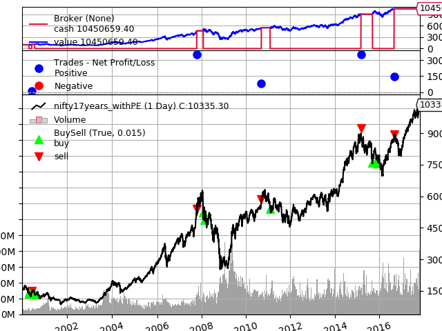
Our strategy is simple, allocate 100% of your funds to NIFTY when P/E ratio of NIFTY is below say 20 and sell all your holdings and cash out if P/E ratio is above 24. Rational - Buy low and sell high and we use P/E estimate how high or low the index is. P/E ratio tells us how undervalued or overvalued the stock/index. Higher the P/E ratio, more overpriced the stock is.

Downloading the data #

Download the data from NSE takes a significan time and you do not want to wait everytime you tweak your strategies. Therefore we download the data and save it to disk.

#%matplotlib inline
from datetime import date
import pandas as pd
try:
    nifty = pd.read_csv('data/nifty17years_withPE.csv')
    print('Read from disk successful')
except:
    print('Downloading from NSE')
    nifty = get_history('NIFTY', date(2000, 1, 1), date(2017, 10, 31), index=True)
    pe = get_index_pe_history('NIFTY', date(2000, 1, 1), date(2017, 10, 31))
    nifty['PE'] = pe['P/E']
    nifty.to_csv('data/nifty17years_withPE.csv')

Load the data in backtrader and run the strategy #

from backtrader.feeds import GenericCSVData

"""
    By default downloaded data only has datetime, Open, High, Low, Close, Volume and Turnover.
    As we are adding one more parameter "PE", we can no longer use GenericCSVData reader provided by 
    backtrader library without modification to base class.
"""
# Define the new parameter
class GenericCSV_PE(GenericCSVData):
    # Add a 'pe' line to the inherited ones from the base class
    lines = ('pe',)
    
    # add the parameter to the parameters inherited from the base class
    params = (('pe', 8),)


# Declare position of each column in csv file
data = GenericCSV_PE(dataname='data/nifty17years_withPE.csv',
                     dtformat=('%Y-%m-%d'),
                     datetime=0,
                     high=1,
                     low=2,
                     open=3,
                     close=4,
                     volume=5,
                     pe=7,
                     openinterest=-1,
                     #fromdate=date(2017,1,1),
                     #todate=date(2017,1,10)
                    )

Defining the strategy #

Defining the strategy described in introduction.

import backtrader as bt


class PEInvesting(bt.SignalStrategy):
    def log(self, txt, dt=None):
        pass

    def __init__(self):
        # Keep a reference to the "close" line in the data[0] dataseries
        self.dataclose = self.datas[0].close
        self.pe = self.datas[0].pe
        

    def next(self):
        curdate = self.datetime.date(ago=0) 
            
        if self.pe[0] < 21:
            self.log(self.dataclose[0])
            # Use 100% of the cash to buy nifty
            self.order_target_percent(target=1.0)
            
       
        if self.pe[0] > 24:
            self.log(self.dataclose[0])
            # Sell everything
            self.order_target_percent(target=0)

Running the defined strategy #

Run the strategy, Get final portfolio value and plot the whole backtesting.

cerebro = bt.Cerebro()

# Set our desired cash start
cerebro.broker.setcash(1000000.0)
cerebro.adddata(data)

cerebro.addstrategy(PEInvesting)
cerebro.run()
print('Final Portfolio Value: %.2f' % cerebro.broker.getvalue())
print('Final value is %.2f times the initial investment'%(cerebro.broker.getvalue()/1000000.0))
cerebro.plot()

output

Next steps #

Play with different possible strategies, eg.

Try different values of PE for buying and selling Try a formula to map relation between P/E value and percentage allocation